Estimation of Obesity Levels Based On Daily Habits
The training dataset provides data for predicting obesity levels in individuals from Mexico, Peru, and Colombia, focusing on their eating habits and physical health.
It encompasses information on 2,111 individuals, leveraging 17 distinct attributes to classify them into various weight categories.
The classification is based on the Body Mass Index (BMI), calculated as BMI = weight (kg) / height2 (m2).
After computing the BMI for each individual, categories were assigned as follows, in alignment with the World Health Organization (WHO) standards:
| Category | BMI Range |
|---|---|
| Underweight | Less than 18.5 |
| Normal | 18.5 to 24.9 |
| Overweight | 25.0 to 29.9 |
| Obesity I | 30.0 to 34.9 |
| Obesity II | 35.0 to 39.9 |
| Obesity III | Higher than 40 |
For more detailed information, please refer to the dataset source, and for an in-depth understanding, consider the introductory paper.
Now calculate your BMI
BMI Calculator
For detailed data analysis and details of how I create the predictive model please refer to details section.
Obesity Prediction Form
Details on the Model and the Data
Data Overview
The dataset encompasses 2,111 individual entries, classifying obesity categories using attributes related
to dietary habits such as frequent consumption of high-caloric foods (FAVC), vegetable consumption
frequency (FCVC), and main meal count (NCP), as well as physical conditions including calorie intake
monitoring (SCC) and technology usage time (TUE), among others.
The following table details these attributes:
| Category | Attribute | Description |
|---|---|---|
| Demographic Information | Gender | The gender of the individual (Female/Male). |
| Age | The age of the individual. | |
| Height | The height of the individual in centimeters. | |
| Weight | The weight of the individual in kilograms. | |
| Eating Habits | FAVC | Frequency of consumption of high caloric food. |
| FCVC | Frequency of vegetable consumption. | |
| NCP | Number of main meals per day. | |
| CAEC | Snacking between main meals. | |
| CH2O | Daily water consumption in liters. | |
| CALC | Alcohol consumption frequency. | |
| Lifestyle Habits | SMOKE | Smoking habit. |
| SCC | Monitoring of calorie intake. | |
| FAF | Physical activity frequency per week. | |
| Technology Use | TUE | Hours spent on technology devices daily. |
| MTRANS | Preferred mode of transportation. | |
| Family History | family_history_with_overweight | Family history of overweight. |
Distribution of the Demographics
In here, the distribution of key demographic features within our dataset, including gender, age, height, and weight, is presented.
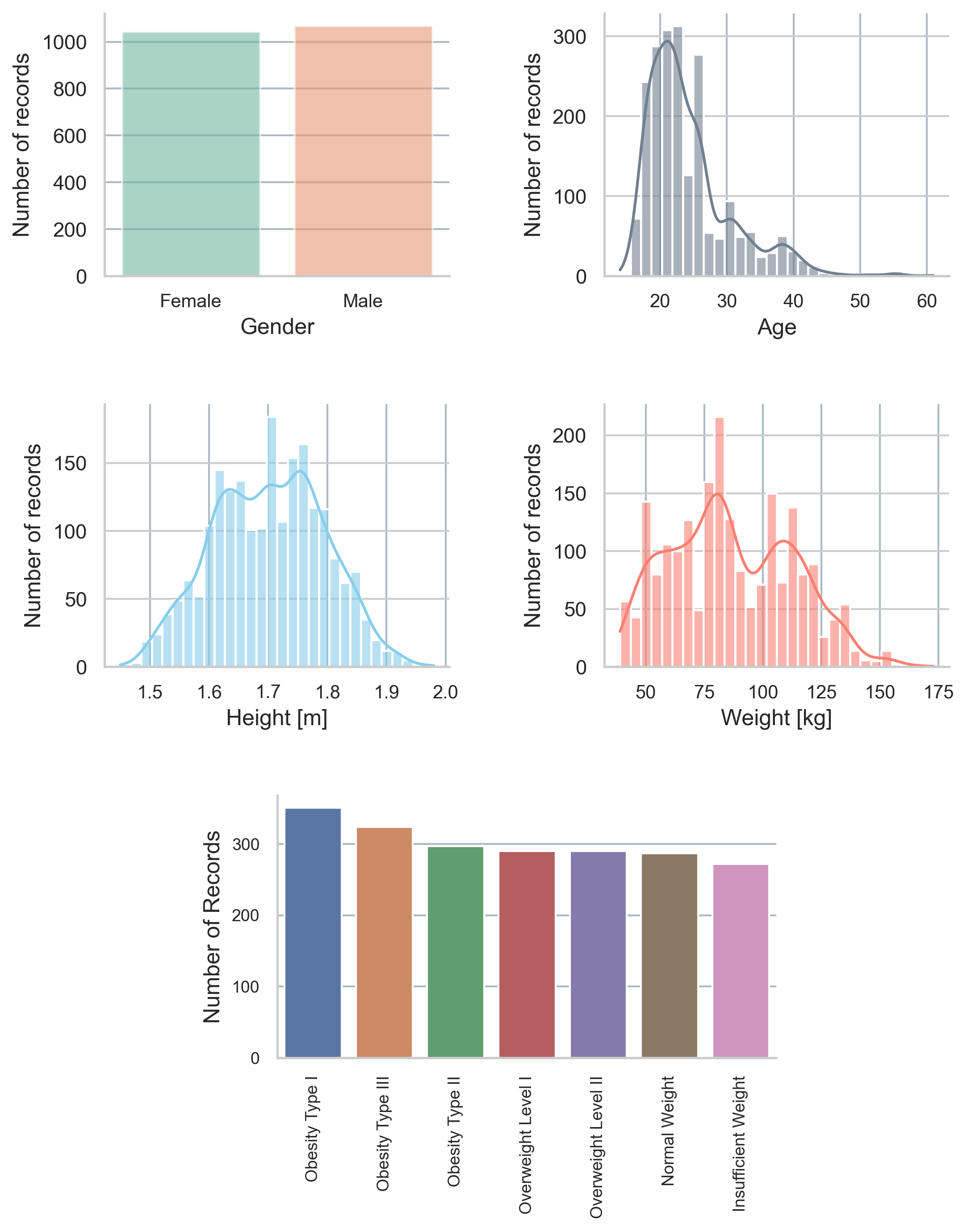
These visualizations highlight the diversity of the dataset, ensuring a comprehensive analysis. The distributions suggest a balanced representation across different demographic groups, laying a solid foundation for fair and accurate obesity category predictions.
This step is crucial in ensuring that any dataset is well-distributed and suitable for further analysis, including feature selection, model training, and evaluation.
Before diving into feature selection for the machine learning predictive model, it is important to explore
and observe potential influences on obesity within the dataset.
One key question to consider is the role of genetics:
does a family history of overweight correlate with increased obesity levels?
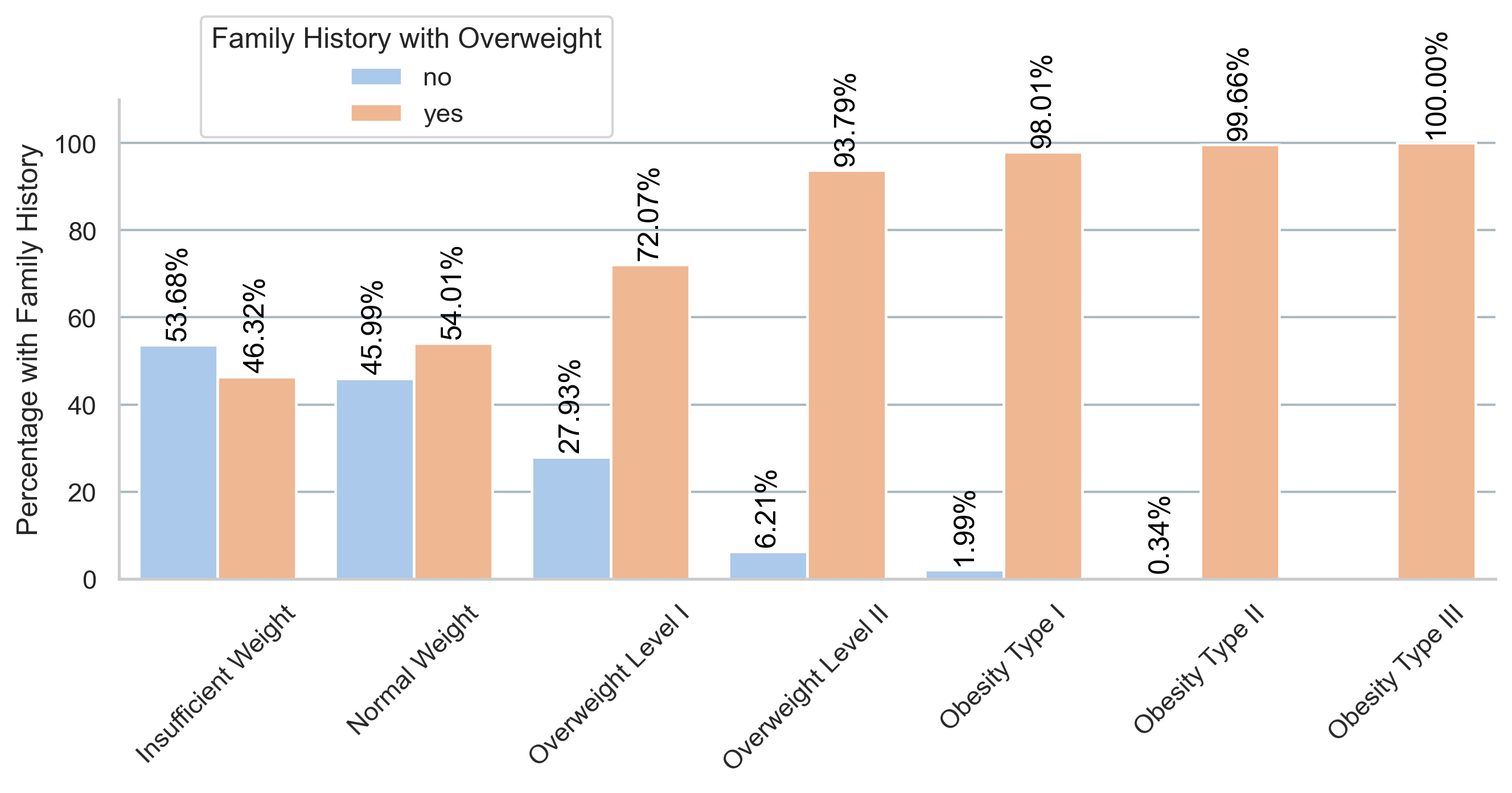
The bar chart above illustrates the relationship between family history and the prevalence of different obesity levels. It indicates a higher proportion of individuals with a family history of overweight in the more severe obesity categories. This pattern suggests that genetic factors may indeed have a significant influence on the likelihood of an individual being overweight or obese. Such insights are valuable for feature selection as they highlight potential predictive variables that could enhance the accuracy of our machine learning model.
As we further prepare the dataset for our predictive modeling, examining lifestyle factors such as daily
water consumption in relation to obesity levels offers additional insights.
It is important to consider whether there's a visible trend or pattern that correlates with the severity of
obesity.
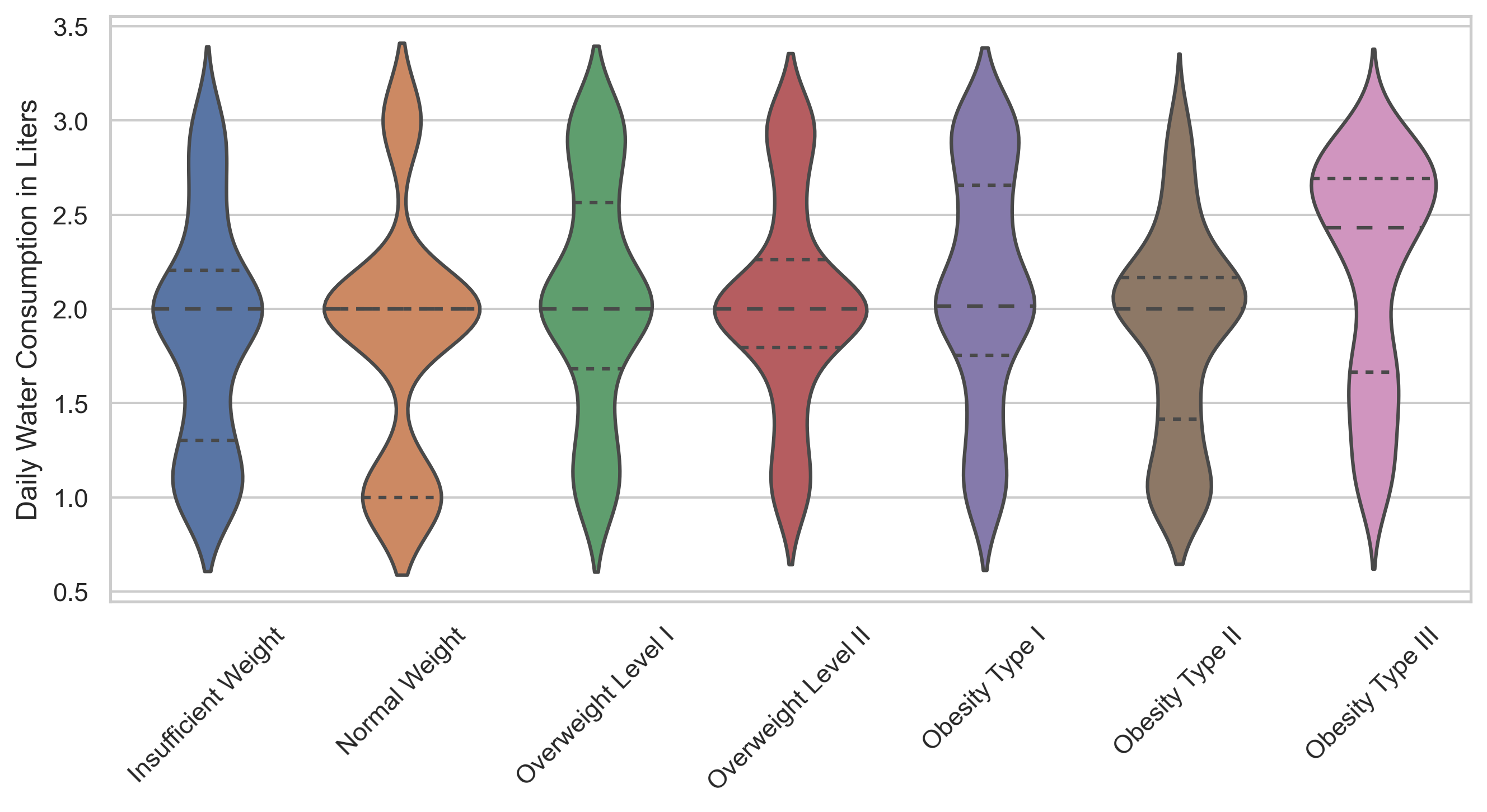
The violin plot above displays the distribution of daily water consumption across different obesity levels.
Each category from 'Insufficient Weight' to 'Obesity Type III' shows variations in water intake. Notably, as
obesity levels increase, the median daily water consumption appears to shift.
This visualization suggests that water consumption patterns may be associated with obesity levels, which
could be a factor to consider in our machine learning model for predicting obesity.
Feature Selection
Moving into the feature selection stage, we aim to refine our dataset by identifying the most influential
variables for predicting obesity levels. This involves discerning which features to encode and normalize to
feed into our predictive models effectively.
We separate our features into categorical and numerical types, apply appropriate transformations, and ready
them for model comparison through cross-validation.
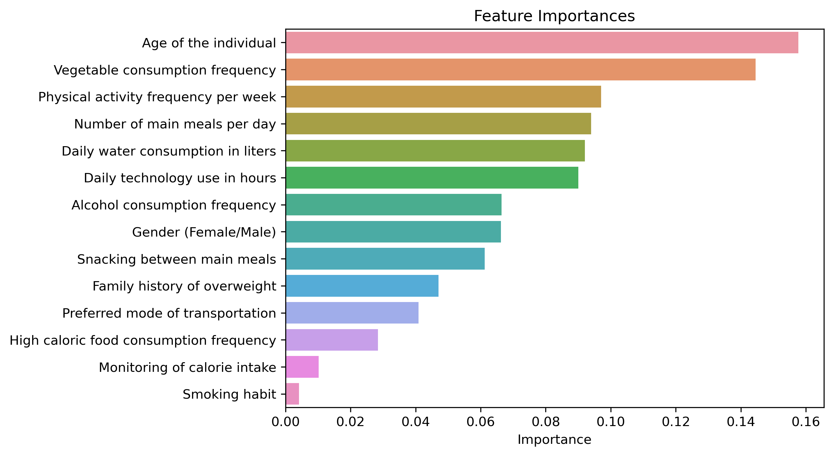
The plot above visualizes the feature importances derived from our Random Forest model, highlighting the variables that most significantly predict obesity levels. Each feature's importance score reflects its contribution to the model's predictive accuracy—higher scores indicate a greater impact. This analysis not only guides our feature selection by identifying the most relevant variables but also underscores the multifactorial nature of obesity, considering a range of demographic, dietary, and lifestyle factors. Such insights are crucial for building a robust model that captures the complexity of obesity prediction.
Model Selection and Training
After identifying the most influential features, the next critical step in our project is model selection and training. This phase involves evaluating various machine learning algorithms to determine which model performs best for our specific dataset and prediction goal. By leveraging a range of models, from simple logistic regression to more complex ensemble methods like Random Forest and Gradient Boosting, we aim to identify the model that not only achieves the highest accuracy but also balances complexity and interpretability. Through systematic comparison and cross-validation, we ensure that our model selection is robust and well-suited for predicting obesity levels.
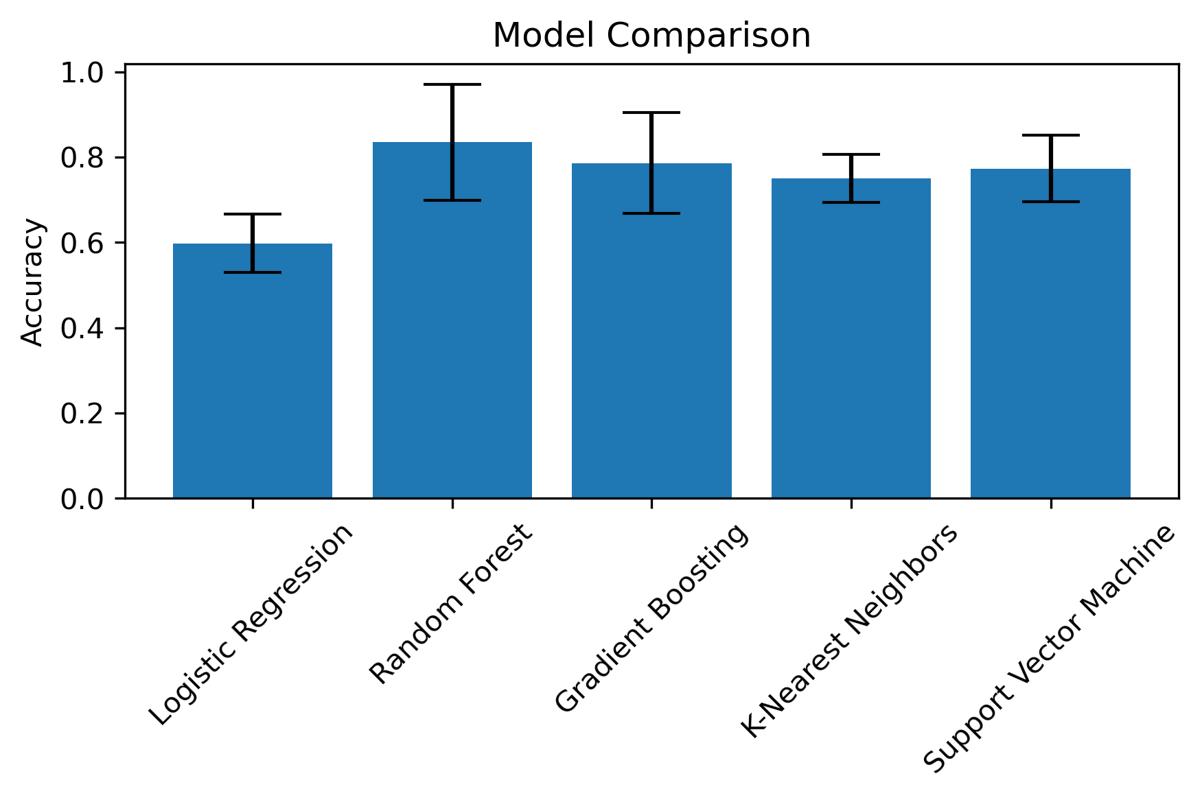
Following a rigorous evaluation through cross-validation, the Random Forest model emerged as the most effective, achieving an average accuracy of 0.83. An accuracy score is a measure of the proportion of correct predictions out of all predictions made.
With the Random Forest model identified as the most promising for our obesity level prediction task, we proceeded to fine-tune its parameters using GridSearchCV. This exhaustive search across a predefined grid of parameters aimed to optimize the model's accuracy by identifying the best combination of settings. The process involved cross-validating each parameter combination to ensure the model's performance was not just a result of overfitting to the training data.
After fine-tuning, the optimized model was then evaluated on a separate test set, which it had not seen during the training or the grid search process. This evaluation step is crucial to assess the model's generalization capability to new, unseen data.
Finally, to demonstrate the practical application of our trained model, we simulated a scenario where we predict the obesity level for a new individual based on a set of hypothetical demographic and lifestyle features. This step showcases how our model can be utilized in real-world applications, providing predictions based on specific input data.
By rigorously tuning and testing our model, and then applying it to both test and hypothetical new data, we have developed a robust tool for predicting obesity levels, which could be further integrated into health assessment platforms or used for educational purposes.